Continuous-Time Transforms – Fourier Transform & Laplace Transform | GATE ECE
Continuous-time transforms provide powerful methods for analyzing signals and systems. Among them, the Fourier Transform and Laplace Transform are closely related and are important topics in GATE ECE.
The Laplace Transform gives a more general representation of a continuous-time signal in the complex-frequency domain. The Fourier Transform can be obtained from the Laplace Transform by putting $s=j\omega$, provided that the Region of Convergence (ROC) includes the imaginary axis.
This relationship makes it easier to understand why the Laplace Transform is useful for a wider range of problems, while the Fourier Transform is mainly used for frequency-domain analysis. In this article, we develop both transforms together so that their connection, properties, and applications become easier to understand and remember.
Keywords: continuous-time transforms, Fourier Transform, CTFT, Laplace Transform, Fourier Transform properties, Laplace Transform properties, inverse Fourier Transform, inverse Laplace Transform, Region of Convergence, ROC, poles and zeros, frequency-domain analysis, GATE ECE signals and systems
The Fourier Transform and Laplace Transform are two closely related tools for continuous-time signal analysis. The key idea is that the Laplace Transform is more general, while the Fourier Transform corresponds to the Laplace Transform evaluated along the imaginary axis.
For the Fourier Transform to exist as the corresponding Laplace-domain representation, the ROC must include the $j\omega$-axis. This connection is especially useful when studying convergence, stability, frequency response, and system behavior.
Fourier Transform
The Fourier Transform converts a continuous-time signal from the time domain into the frequency domain. It shows how different frequency components are present in the signal and is useful for studying its spectrum, magnitude, phase, and bandwidth.
Fourier Transform Forms of $x(t)$
Fourier Transform:
$X(\omega)=\int_{-\infty}^{\infty}x(t)e^{-j\omega t}\,dt$
Inverse Fourier Transform:
$x(t)=\frac{1}{2\pi}\int_{-\infty}^{\infty}X(\omega)e^{j\omega t}\,d\omega$
Note: The Hilbert Transform of x(t) is obtained by multiplying its Fourier Transform by $-j\,\mathrm{sgn}(\omega)$:
$\mathcal{F}\{\hat{x}(t)\}=-j\,\mathrm{sgn}(\omega)\,X(\omega)$
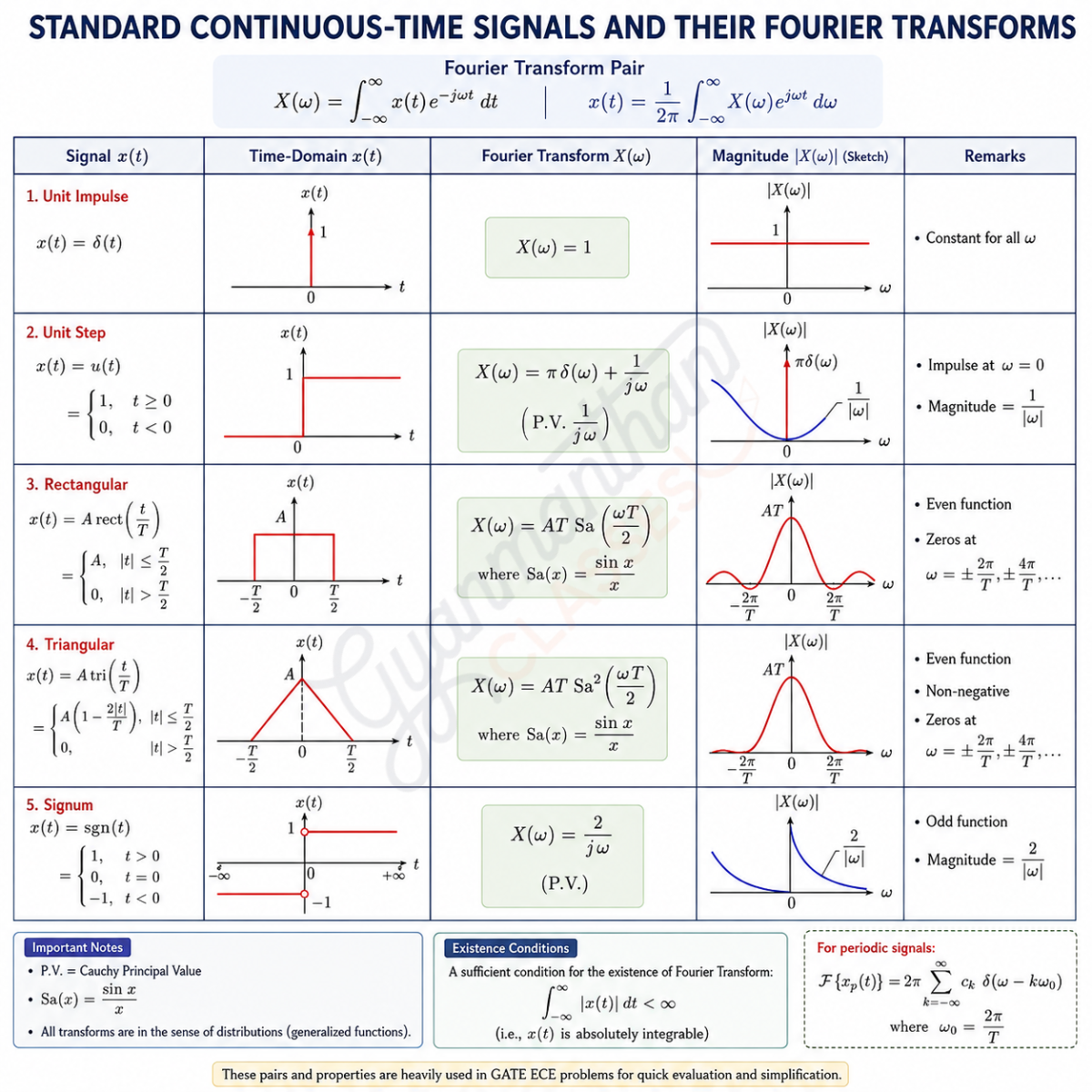
Key Characteristics
- The Fourier Transform converts a continuous-time signal from the time domain to the frequency domain.
- $X(\omega)$ represents the frequency components present in the signal $x(t)$.
- The inverse Fourier Transform reconstructs $x(t)$ from $X(\omega)$.
- For a periodic signal, the Fourier Transform consists of impulses located at the harmonic frequencies.
- Signal properties such as linearity, time shifting, scaling, differentiation, and convolution can be used to simplify Fourier Transform calculations.
- For a Laplace Transform with an ROC that includes the imaginary axis, the Fourier Transform is obtained by setting $s=j\omega$.
- Standard Fourier Transform pairs such as $\delta(t)$, $u(t)$, rectangular and triangular pulses are frequently useful in GATE problems.
- Using the appropriate transform property or standard pair can significantly reduce the calculation required in GATE problems.
Laplace Transform
The Laplace Transform extends the idea of frequency-domain analysis to the complex-frequency domain. It is particularly useful for analyzing differential equations, transient behavior, system stability, poles, zeros, and system response.
Laplace Transform of x(t):
Laplace Transform:
$X(s)=\int_{-\infty}^{\infty}x(t)e^{-st}\,dt$
Inverse Laplace Transform:
$x(t)=\frac{1}{2\pi j}\int_{\gamma-j\infty}^{\gamma+j\infty}X(s)e^{st}\,ds$
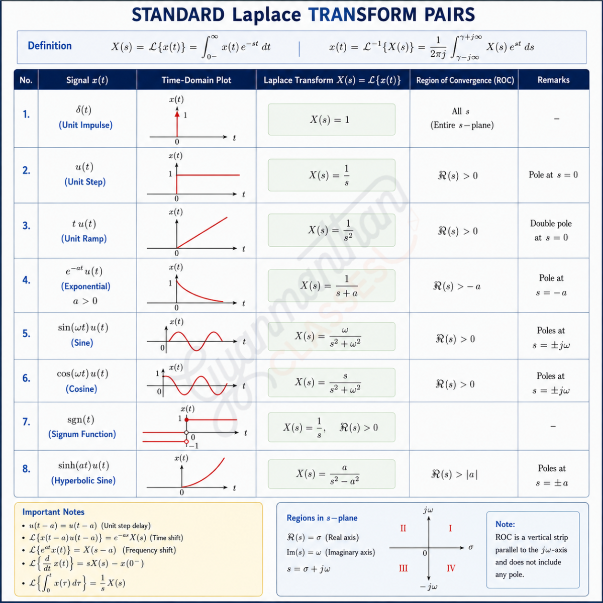
Important Properties of ROC
- The Region of Convergence (ROC) is the set of values of $s$ for which the Laplace Transform converges.
- For a rational Laplace Transform, the ROC is a vertical half-plane or vertical strip in the $s$-plane.
- The ROC never contains any pole of $X(s)$.
- For a right-sided signal, the ROC lies to the right of the rightmost pole.
- For a left-sided signal, the ROC lies to the left of the leftmost pole.
- For a two-sided signal, the ROC lies between two poles and forms a vertical strip.
- For a combination of right-sided components, the ROC extends to the right of the rightmost pole.
- For a combination of left-sided components, the ROC extends to the left of the leftmost pole.
- For a combination of right-sided and left-sided signals, the ROC exists only if the rightmost pole of the right-sided component lies to the left of the leftmost pole of the left-sided component.
- If the individual ROCs have no common region, the Laplace Transform does not exist.
- A signal is stable if its ROC includes the imaginary axis ($s=j\omega$).
- If the ROC includes the imaginary axis, the Fourier Transform exists under the usual convergence conditions.
- For a causal rational system, the ROC lies to the right of the rightmost pole.
- For a causal and stable rational system, all poles lie in the left half of the $s$-plane.
- The ROC together with $X(s)$ uniquely determines the corresponding time-domain signal.
Relation Between Laplace and Fourier Transform
The Laplace Transform is defined using $s=\sigma+j\omega$. When $\sigma=0$, we have $s=j\omega$, which corresponds to the imaginary axis. Therefore, the Fourier Transform is obtained from the Laplace Transform by evaluating it on the imaginary axis:
$X(\omega)=X(s)\big|_{s=j\omega}$
For the Fourier Transform to exist, the imaginary axis must lie within the ROC of the Laplace Transform. Since the ROC never contains poles, there must be no pole on the imaginary axis.
Fourier Transform Properties:
| Property | Time Domain | Frequency Domain |
|---|---|---|
| Linearity | $ax_1+bx_2$ | $aX_1+bX_2$ |
| Time Shifting | $x(t-t_0)$ | $e^{-j\omega t_0}X(\omega)$ |
| Frequency Shifting | $x(t)e^{j\omega_0t}$ | $X(\omega-\omega_0)$ |
| Time Scaling | $x(at)$ | $\frac{1}{|a|}X(\frac{\omega}{a})$ |
| Time Differentiation | $\frac{dx(t)}{dt}$ | $j\omega X(\omega)$ |
| Convolution | $x(t)*h(t)$ | $X(\omega)H(\omega)$ |
| Multiplication | $x(t)h(t)$ | $\frac{1}{2\pi}X(\omega)*H(\omega)$ |
| Parseval | $\int|x(t)|^2dt$ | $\frac{1}{2\pi}\int|X(\omega)|^2d\omega$ |
Laplace Transform Properties:
| Property | Time Domain | Laplace Domain |
|---|---|---|
| Linearity | $ax_1+bx_2$ | $aX_1+bX_2$ |
| Time Shifting | $x(t-t_0)$ | $e^{-st_0}X(s)$ |
| Time Differentiation | $\frac{dx(t)}{dt}$ | $sX(s)-x(0^-)$ |
| Time Integration | $\int_{-\infty}^{t}x(\tau)d\tau$ | $\frac{X(s)}{s}$ |
| Convolution | $x(t)*h(t)$ | $X(s)H(s)$ |
| Multiplication by $t$ | $tx(t)$ | $-\frac{dX(s)}{ds}$ |
| Initial Value | $\lim_{t\to0^+}x(t)=\lim_{s\to\infty}sX(s)$ | |
| Final Value | $\lim_{t\to\infty}x(t)=\lim_{s\to0}sX(s)$ | |
| ROC | Determines convergence | |




Discussion / Comments